Chapter 2 Euclidean Space

2.1 Algebra: Vectors

Theorem 2.1.1 (Vector space axioms).

(A1) Addition is associative

(A2) 0 is an additive identity

(A3) Existence of additive inverses

(A4) Addition is commutative

(M1) Scalar multiplication is associative

(M2) 1 is a multiplicative identity

(D1) Scalar multiplication distributes over scalar addition

(D2) Scalar multiplication distributes over vector addition

For $n > 1$, $\mathbb{R}^n$ is not endowed with vector-by-vector multiplication.

If the vector space axioms are satisfied with $V$ and $F$ replacing $\mathbb{R}^n$ and $\mathbb{R}$ then we say that $V$ is a vector space over $F$.

We can use intrinsic vector algebra to prove a result from Euclidean geometry, that the three medians of a triangle intersect.

Let

$$p = \frac{x + y + z}{3}$$

Rewrite it as

$$p = x + \frac{2}{3}(\frac{y+z}{2} - x)$$

Note that $\frac{y+z}{2}$ is the middle point of $yz$. Then $\frac{y+z}{2} - x$ is the median from $x$ to $yz$, so $p$ is on the median.

Since $x,y,z$ are symmetric, then $p$ is on all 3 medians.

$\square$

The standard basis of $\mathbb{R}^n$ is the set of vectors

$$e_1 = (1, 0, \cdots 0) \\ e_2 = (0, 1, \cdots 0) \\ \cdots \\ e_n = (0, 0, \cdots 1) \\ $$

So

$$\tag{2.1} x = \sum_{i = 1}^{n}x_i e_i$$

Definition 2.1.2 (Basis).

A set of vectors $\{f_i\}$ is a basis of $\mathbb{R}^n$ if every $x ∈ \mathbb{R}^n$ is uniquely expressible as a linear combination of the $f_i$.

$\square$

2.2 Geometry: Length and Angle

Definition 2.2.1 (Inner product).

The inner product is a function from pairs of vectors to scalars,

$$\left\langle , \right\rangle : \mathbb{R}^n \times \mathbb{R}^n \rightarrow \mathbb{R}$$

defined by the formula

$$\left\langle (x_1, \cdots, x_n) , (y_1, \cdots, y_n) \right\rangle = \sum_{i = 1}^{n} x_i y_i$$

Proposition 2.2.2 (Inner product properties).

(IP1) The inner product is positive definite: $⟨x,x⟩ ≥ 0$ for all $x ∈ \mathbb{R}^n$, with equality if and only if $x = 0$.

(IP2) The inner product is symmetric: $⟨x,y⟩= ⟨y,x⟩$ for all $x,y ∈ \mathbb{R}^n$

(IP3) The inner product is bilinear:

$$⟨x+x',y⟩ = ⟨x,y⟩ + ⟨x',y⟩, \quad ⟨ax,y⟩ = a ⟨x,y⟩ \\ ⟨x,y+y'⟩ = ⟨x,y⟩ + ⟨x,y'⟩, \quad ⟨x,by⟩ = b ⟨x,y⟩$$

for all $a,b ∈ \mathbb{R}$, $x,x',y,y' ∈ \mathbb{R}^n$.

$\square$

Like the vector space axioms, the inner product properties are phrased intrinsically, although they need to be proved using coordinates. As mentioned in the previous section,intrinsic methods are neater and more conceptual than using coordinates. More importantly:

The rest of the results of this section are proved by reference to the inner product properties, with no further reference to the inner product formula.

Definition 2.2.3 (Modulus).

The modulus (or absolute value) of a vector $x ∈ \mathbb{R}^n$ is defined as

$$|x| = \sqrt[]{⟨x,x⟩}.$$

Proposition 2.2.4 (Modulus properties).

(Mod1) The modulus is positive: $|x| ≥ 0$ for all $x ∈ \mathbb{R}^n$, with equality if and only if $x = 0$.

(Mod2) The modulus is absolute-homogeneous: $|ax|= |a||x|$ for all $a ∈ R$ and $x ∈ \mathbb{R}^n$.

Theorem 2.2.5 (Cauchy–Schwarz inequality).

For all $x,y ∈ \mathbb{R}^n$,

$$|⟨x,y⟩| \leq |x| |y|$$

with equality if and only if one of $x, y$ is a scalar multiple of the other.

Note that the absolute value signs mean different things on each side of the Cauchy–Schwarz inequality. On the left side, the quantities $x$ and $y$ are vectors, their inner product $⟨x,y⟩$ is a scalar, and $|⟨x,y⟩|$ is its scalar absolute value, while on the right side, $|x|$ and $|y|$ are the scalar absolute values of vectors, and $|x||y|$ is their product. That is, the Cauchy–Schwarz inequality says:

The size of the product is at most the product of the sizes.

The computation draws on the minutiae of the formulas for the inner product and the modulus, rather than using their properties. It is uninformative, making the Cauchy–Schwarz inequality look like a low-level accident. It suggests that larger-scale mathematics is just a matter of bigger and bigger formulas. To prove the inequality in a way that is enlightening and general, we should work intrinsically, keeping the scalars $⟨x,y⟩$ and $|x|$ and $|y|$ notated in their concise forms, and we should use properties, not formulas.

Proof. The result is clear when $x = 0$, so assume $x \neq 0$. For every $a ∈ \mathbb{R}^n$,

$$\begin{split} 0 &\leq ⟨ax-y,ax-y⟩ \quad \\ & \quad \text{by positive definiteness} \\ &= a⟨x,ax-y⟩ - ⟨y,ax-y⟩ \\ & \quad \text{by linearity in the first variable} \\ &= a^2 ⟨x,x⟩ - a ⟨x,y⟩ - a ⟨y,x⟩ + ⟨y,y⟩ \\ & \quad \text{by linearity in the second variable} \\ &= a^2 |x|^2 - 2a ⟨x,y⟩ + |y|^2 \\ & \quad \text{by symmetry, definition of modulus.} \end{split}$$

Define

$$f(a) = a^2 |x|^2 - 2a ⟨x,y⟩ + |y|^2$$

Since $f(a)$ is always nonnegative, so $f$ has at most one root. Thus by the quadratic formula its discriminant is nonpositive,

$$4⟨x,y⟩^2 −4|x|^2|y|^2 ≤ 0$$

So

$$|⟨x,y⟩| \leq |x| |y|$$

Equality holds exactly when the quadratic polynomial $f(a) = |ax− y|^2$ has a root a, i.e., exactly when $y= ax$ for some $a ∈ \mathbb{R}^n$.

$\square$

Theorem 2.2.6 (Triangle inequality).

For all $x,y ∈ \mathbb{R}^n$,

$$|x+y| \leq |x| + |y|,$$

with equality if and only if one of $x, y$ is a nonnegative scalar multiple of the other.

Proof:

$$\begin{split} ⟨x+y,x+y⟩ \\ &= ⟨x,x+y⟩ + ⟨y,x+y⟩ \\ &= ⟨x,x⟩ + ⟨x,y⟩ + ⟨y,x⟩ + ⟨y,y⟩ \\ &= ⟨x,x⟩ + 2⟨x,y⟩ + ⟨y,y⟩ \\ &\leq ⟨x,x⟩ + 2|x||y| + ⟨y,y⟩ \\ & \quad \text{by Cauchy–Schwarz} \\ &= (|x| + |y|)^2 \end{split}$$

Equality holds exactly when $⟨x,y⟩= |x||y|$, or equivalently when $|⟨x,y⟩|= |x||y|$ and $⟨x,y⟩ ≥ 0$. These hold when one of $x, y$ is a scalar multiple of the other and the scalar is nonnegative.

$\square$

• While the Cauchy–Schwarz inequality says that the size of the product is at most the product of the sizes, the triangle inequality says:

The size of the sum is at most the sum of the sizes.

Proposition 2.2.7 (Size bounds).

For every $j ∈ \{1,...,n\}$,

$$|x_j| \leq |x| \leq \sum_{i=1}^{n} |x_i|.$$

Distance Definition

The modulus gives rise to a distance function on Rn that behaves as distance should. Define

$$d: \mathbb{R}^n \times \mathbb{R}^n \xrightarrow{} \mathbb{R}$$

by

$$d(x,y) = |y-x|$$

Theorem 2.2.8 (Distance properties).

(D1) Distance is positive: $d(x,y) ≥ 0$ for all $x,y ∈ \mathbb{R}^n$, and $d(x,y) = 0$ if and only if $x = y$.

(D2) Distance is symmetric: $d(x,y) = d(y,x)$ for all $x,y ∈ \mathbb{R}^n$.

(D3) Triangle inequality: $d(x,z) ≤ d(x,y)+d(y,z)$ for all $x,y,z ∈ \mathbb{R}^n$.

Angle Definition

If $x$ and $y$ are nonzero vectors in $\mathbb{R}^n$, define their angle $θ_{x,y}$ by the condition

$$\tag{2.2} \cos θ_{x,y} = \frac{⟨x,y⟩}{|x||y|}, \quad 0 \leq θ_{x,y} \leq π.$$

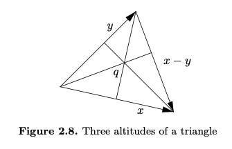
In particular, two nonzero vectors $x$ and $y$ are orthogonal when $⟨x,y⟩ = 0$. Thus $0$ orthogonal to all vectors.

three altitudes must meet

We have

$$q-y \perp x \quad \text{and} \quad q-x \perp y$$

And we want to show

$$\left\{ \begin{array}{lr} ⟨q-y,x⟩ = 0 \\ ⟨q-x,y⟩ = 0 \\ \end{array} \right\} \Longrightarrow ⟨q,x-y⟩ = 0$$

We have

$$\left\{ \begin{array}{lr} ⟨q,x⟩ - ⟨y,x⟩ = 0 \\ ⟨q,y⟩ - ⟨x,y⟩ = 0 \\ \end{array} \right\} \Longrightarrow ⟨q,x-y⟩ = 0$$

So we have

$$⟨q,x⟩ = ⟨y,x⟩ = ⟨x,y⟩ = ⟨q,y⟩ \\ \Longrightarrow \\ ⟨q,x-y⟩ = 0$$

$\square$

2.3 Analysis: Continuous Mappings

Mapping from $\mathbb{R}^n$ to $\mathbb{R}^m$

A mapping from $\mathbb{R}^n$ to $\mathbb{R}^m$ is some rule that assigns to each point $x$ in $\mathbb{R}^n$ a point in $\mathbb{R}^m$. Generally, mappings will be denoted by letters such as $f, g, h$.

Mappings as a vector space

For a given dimension $n$, a given set $A ⊂ \mathbb{R}^n$, and a second dimension $m$, let $\mathcal{M}(A,\mathbb{R}^m)$ denote the set of all mappings $f : A \rightarrow \mathbb{R}^m$. This set forms a vector space over $\mathbb{R}$ (whose points are functions) under the operations

$$+ : \mathcal{M}(A,\mathbb{R}^m) \times \mathcal{M}(A,\mathbb{R}^m) \longrightarrow \mathcal{M}(A,\mathbb{R}^m),$$

defined by

$$(f +g)(x) = f(x)+g(x) \quad\text{for all } x ∈ A,$$

and

$$\cdot : \mathbb{R} \times \mathcal{M}(A,\mathbb{R}^m) \longrightarrow \mathcal{M}(A,\mathbb{R}^m),$$

defined by

$$(a \cdot f )(x) = a \cdot f(x) \quad\text{for all } x ∈ A.$$

Sequence in $\mathbb{R}^n$

Let $A$ be a subset of $\mathbb{R}^n$. A sequence in $A$ is an infinite list of vectors $\{x_1,x_2,x_3,...\}$ in $A$, often written $\{x_ν\}$.

Since a vector has $n$ entries, each vector $x_ν$ in the sequence takes the form $(x_{1,ν},...,x_{n,ν})$.

Definition 2.3.1 (Null Sequence).

The sequence $(x_{\nu })$ in $\mathbb{R}^n$ is null if for every $ε > 0$ there exists some $ν_0$ such that

$$\text{if } ν > ν_0 \text{ then } |x_v| < \epsilon.$$

That is, a sequence is null if for every $ε > 0$, all but finitely many terms of the sequence lie within distance $ε$ of $0_n$.

• If $\{x_ν\}$ is a null sequence and $|y_ν| \leq |x_ν|$ or all $ν$ then also $\{y_ν\}$ is null.
• $\{x_ν\}$ and $\{y_ν\}$ are null sequence, then $|x_ν + y_ν| \leq |x_ν| + |y_ν|$, so $\{x_ν + y_ν\}$ is null.
• $\{c x_ν\}$ is null seq, since $|cx_ν| = |c||x_ν|$

So the set of null sequences in $\mathbb{R}^n$ forms a vector space.

A vector sequence $\{x_ν\}$ is null if and only if the scalar sequence $\{|x_ν|\}$ is null.

Lemma 2.3.2 (Componentwise nature of nullness).

The vector sequence $\{(x_{1,ν}, \cdots, x_{n,ν})\}$ is null if and only if each of its component scalar sequences $\{x_{j,ν}\} (j \in \{1, \cdots, n\})$ is null.

Proof

Use

$$|x_{j,ν}| \leq |x_ν| \leq \sum_{j=1}^{n} |x_{j,ν}|$$

$\square$

Definition 2.3.3 (Sequence convergence, sequence limit).

Let $A$ be a subset of $\mathbb{R}^n$. Consider a sequence $\{x_ν\}$ in $A$ and a point $p ∈ \mathbb{R}^n$. The sequence $\{x_ν\}$ converges to $p$ (or has limit $p$), written $\{x_ν\} → p$, if the sequence $\{x_ν−p\}$ is null. When the limit $p$ is a point of $A$, the sequence $\{x_ν\}$ converges in $A$.

A sequence can only converges to one limit.

Proposition 2.3.4 (Linearity of convergence).

Let $\{x_ν\}$ be a sequence in $\mathbb{R}^n$ converging to $p$, let $\{y_ν\}$ be a sequence in $\mathbb{R}^n$ converging to $q$, and let $c$ be a scalar. Then the sequence $\{x_ν +y_ν\}$ converges to $p+q$, and the sequence $\{c x_ν\}$ converges to $c_p$.

Proof:

$$\begin{split} |(x_ν + y_ν) - (p + q)| &= |(x_ν - p) + (y_ν-q)| \\ &\leq |x_ν - p| + |y_ν - q| \end{split}$$

So $(x_ν + y_ν) - (p + q)$ is null. Then $x_ν + y_ν → p+q$.

$$|c x_ν - cp| = |c (x_ν - p)| \leq |c| |x_ν - p|$$

So $c x_ν - cp$ is null. Then $c x_ν → cp$

$\square$

Proposition 2.3.5 (Componentwise nature of convergence).

The vector sequence $\{(x_{1, ν}, \cdots, x_{n, ν})\}$ converges to the vector $(p_1, \cdots, p_n)$ if and only if each component scalar sequence $\{x_{j, ν}\} (j = 1, \cdots, n)$. converges to the scalar $p_j$.

Proof:

$$\{(x_{1, ν}, \cdots, x_{n, ν})\} \longrightarrow p \\ \Longleftrightarrow \\ x_ν - p \quad \text{is null} \\ \Longleftrightarrow \\ x_{j, ν} - p_j \quad \text{is null} \\ \Longleftrightarrow \\ x_{j, ν} \longrightarrow p_j$$

$\square$

Definition 2.3.6 (Continuity).

Let $A$ be a subset of $\mathbb{R}^n$, let $f : A \longrightarrow \mathbb{R}^m$ be a mapping, and let $p$ be a point of $A$. Then $f$ is continuous at $p$ if for every sequence $\{x_ν\}$ in $A$ converging to $p$, the sequence $f(x_ν)$ converges to $f(p)$. The mapping $f$ is continuous on $A$ (or just continuous when $A$ is clearly established) if it is continuous at each point $p ∈ A$.

Modulus function is continuous

$$|| : \mathbb{R}^n \longrightarrow \mathbb{R}$$

Proof:

Assume $\{x_ν\} \rightarrow p$, then from exercise 2.2.7

$$||x_ν| - |p|| \leq | x_ν - p |$$

Then $|x_ν| - |p|$ is null, i.e. $\{f(x_ν)\} \rightarrow f(p)$. So $||$ is continuous.

The inner product is continuous

Given $a \in \mathbb{R}^n$, define

$$T : \mathbb{R}^n \longrightarrow \mathbb{R}^n, \quad T(x) = ⟨a,x⟩$$

$T$ is continuous.

From Cauchy-Schwarz inequality

$$|⟨a,x⟩| \leq |a||x|$$

Given $p \in \mathbb{R}^n$ $$|T(x_ν) - T(p)| = |⟨a,x_v⟩ - ⟨a,p⟩| = |⟨a,x_ν - p⟩| \leq |a| | x_ν - p |$$

Since we know $|x_ν - p| \rightarrow 0$, we have $|T(x_ν) - T(p)| \rightarrow 0$.

$\square$

jth coordinate function map

Consider the following mapping

$$\pi_j : \mathbb{R}^n \longrightarrow \mathbb{R}, \quad \pi_j (x_1, \cdots, x_n) = x_j$$

Since $\pi_j(x) = ⟨e_j,x⟩$, this mapping is continuous.

Proposition 2.3.7 (Vector space properties of continuity).

Let $A$ be a subset of $\mathbb{R}^n$, let $f,g : A \longrightarrow \mathbb{R}^m$ be continuous mappings, and let $c \in \mathbb{R}$. Then the sum and the scalar multiple mappings

$$f+g,cf : A \longrightarrow \mathbb{R}^m$$

are continuous. Thus the set of continuous mappings from $A$ to $\mathbb{R}^m$ forms a vector subspace of $\mathcal{M}(A, \mathbb{R}^m)$.

Proof:

Given $p \in A$, and $\{x_ν\} \rightarrow p$. Then $\{f(x_ν)\} \rightarrow f(p), \{g(x_ν)\} \rightarrow g(p)$.

Then from Proposition 2.3.4 (Linearity of convergence), $\{f(x_ν) + g(x_ν)\} \rightarrow f(p) + g(p)$, i.e. $\{(f+g)(x_ν)\} \rightarrow (f+g)(p)$. So $f+g$ is continuous.

For the same reason $cf$ is continuous.

$\square$

Proposition 2.3.8 (Persistence of continuity under composition).

Let $A$ be a subset of $\mathbb{R}^n$, let $f : A \longrightarrow \mathbb{R}^m$ be a continuous mapping.

Let $B$ be a superset of $f(A)$ in $\mathbb{R}^m$, and let $g : B \longrightarrow \mathbb{R}^l$ be a continuous mapping.

Then the composition mapping

$$g \circ f : A \longrightarrow \mathbb{R}^l$$

is continuous.

Proof:

Given $p \in A$, and $\{x_ν\} \rightarrow p$. We have $\{f(x_ν)\} \rightarrow f(p)$.

Since $f(x_ν), f(p) \in B$, and $g$ is a continuous mapping, we have $\{g(f(x_ν))\} \rightarrow g(f(p))$.

Therefore, $g \circ f$ is continuous.

$\square$

Theorem 2.3.9 (Componentwise nature of continuity).

Let $A ⊂ \mathbb{R}^n$, let $f : A \longrightarrow \mathbb{R}^m$ have component functions $f_1,...,f_m$, and let $p$ be a point in $A$. Then

$$f \text{ is continuous at } p \Longleftrightarrow \text{each } f_i \text{ is continuous at } p.$$

Proof:

$\Rightarrow$

Given any sequence $(x_{\nu}) \rightarrow p$, since $f$ is continuous at $p$, then $f(x_{\nu}) \rightarrow f(p)$.

From Proposition 2.3.5 Componentwise nature of convergence $f_i(x_{\nu}) \rightarrow f_i(p)$.

So $f_i$ is continuous at $p$.

$\Leftarrow$

Given any sequence $(x_{\nu}) \rightarrow p$, and since $f_i$ is continuous at $p$, then $f_i(x_{\nu}) \rightarrow f_i(p)$.

From Proposition 2.3.5 Componentwise nature of convergence $f(x_{\nu}) \rightarrow f(p)$.

So $f$ is continuous at $p$.

$\square$

Some examples

Consider

$$f(x, y) = \begin{cases} \frac{2xy}{x^2 + y^2} &\text{if } (x,y) \neq 0\\ b &\text{if } (x,y) = 0\\ \end{cases}$$

Can the constant $b$ be specified to make $f$ continuous at $0$?

Take a sequence $\{(x_ν, y_ν)\} \rightarrow 0$ along the line $y= mx$.

$$f(x_ν, y_ν) = \\ \frac{2x_ν y_ν}{x_ν^2 + y_ν^2} = \\ \frac{2m}{1 + m^2}$$

hence $f$ cannot be made continuous at $0$.

$\square$

Now consider

$$g(x, y) = \begin{cases} \frac{x^2y}{x^4 + y^2} &\text{if } (x,y) \neq 0\\ b &\text{if } (x,y) = 0\\ \end{cases}$$

If $(x,y)$ approaches to $(0,0)$ with $y = x$, then

$$g(x,y) = \frac{x^3}{x^4 + x^2} = \frac{x}{x^2 + 1} \rightarrow 0$$

If $(x,y)$ approaches to $(0,0)$ with $y = x^2$, then

$$g(x,y) = \frac{x^4}{x^4 + x^4} = \frac{1}{2}$$

hence $f$ cannot be made continuous at $0$.

$\square$

The size bounds to prove continuity

Consider

$$h(x, y) = \begin{cases} \frac{x^3}{x^2 + y^2} &\text{if } (x,y) \neq 0\\ b &\text{if } (x,y) = 0\\ \end{cases}$$

Note from 2.2.7, we have $|x| \leq |(x,y)|$, so $$\frac{x^3}{x^2 + y^2} \leq \frac{|(x,y)|^3}{|(x,y)|^2} = |(x,y)| \rightarrow 0$$

So setting $b = 0$ makes it continuous at $0$.

Summary of the 3 examples

The straight line test can prove that a limit does not exist, or it can determine the only candidate for the value of the limit, but it cannot prove that the candidate value is the limit.

When the straight line test determines a candidate value of the limit, approaching along a curve can further support the candidate, or it can prove that the limit does not exist by determining a different candidate as well.

The size bounds can prove that a limit does exist, but they can only suggest that a limit does not exist.

Proposition 2.3.10 (Persistence of inequality).

Let $A$ be a subset of $\mathbb{R}^n$ and let $f : A \longrightarrow \mathbb{R}^m$ be a continuous mapping. Let $p$ be a point of $A$, let $b$ be a point of $\mathbb{R}^m$, and suppose that $f(p) \neq b$. Then there exists some $\epsilon > 0$, such that

$$\text{for all } x \in A \text{such that } |x-p| < \epsilon, f(x) \neq b.$$

Proof:

Assume otherwise, then for $\nu \in \mathbb{N}$, we can find $x_ν$, such that $| x_ν - p | < 1/ν$ and $f(x_ν) = b$.

Since $f$ is continuous, then $f(p) = b$. We have a contradiction.

$\square$

2.4 Topology: Compact Sets and Continuity

Definition 2.4.1 (ε-ball).

For every point $p ∈ \mathbb{R}^n$ and every positive real number $ε > 0$, the $ε$-ball centered at $p$ is the set

$$B(p, ε) = \{x \in \mathbb{R}^n : |x-p| \leq ε\}$$

Definition 2.4.2 (Limit point).

Let $A$ be a subset of $\mathbb{R}^n$, and let $p$ be a point of $\mathbb{R}^n$. The point $p$ is a limit point of A if every $ε$-ball centered at $p$ contains some point $x ∈ A$ such that $x \neq p$.

Isolated point

Definition 1: A point in $A$ that is not a limit point of $A$.

Definition 2: Equivalently, $p$ is an isolated point of $A$ if $p ∈ A$ and there exists some $ε > 0$ such that $B(p,ε)∩A= \{p\}$.

Lemma 2.4.3 (Sequential characterization of limit points).

Let $A$ be a subset of Rn, and let $p$ be a point of $\mathbb{R}^n$. Then $p$ is the limit of a sequence $\{x_ν\}$ in $A$ with each $x_ν \neq p$ if and only if $p$ is a limit point of $A$.

Proof:

$\Rightarrow$

Given $B(p, ε)$, since $\{x_ν\} \rightarrow p$, we can find $ν_0$, such that $ν > ν_0$, $|x_ν - p| < ε$, i.e. $x_ν \in B(p, ε)$. Since $x_ν \neq p$, then $p$ is a limit point of $A$.

$\Leftarrow$

Assume $p$ is a limit point of $A$, let $x_1 \in A$. Let $ε_1 = |x_1 - p|$, and $ε_2 = ε_1 / 2$. We can find $p \neq x_2 \in B(p, ε_2)$. This process can continue infinitely. Then we find a $\{x_ν\} \rightarrow p$.

$\square$

Definition 2.4.4 (Closed set).

A subset $A$ of $\mathbb{R}^n$ is closed if it contains all of its limit points.

Proposition 2.4.5 (Sequential characterization of closed sets).

Let $A$ be a subset of $\mathbb{R}^n$. Then $A$ is closed if and only if every sequence in $A$ that converges in $\mathbb{R}^n$ in fact converges in $A$.

Proof:

$\Rightarrow$

Assume $\{x_ν\} \rightarrow p$ and $x_ν \in A$, if $p = x_ν$ for some $ν$, then $p \in A$.

If $p \neq x_ν$, then $p$ is a limit point of $A$. Since $A$ is closed, so $p \in A$.

$\square$

$\Leftarrow$

Assume $p$ is a limit point of $A$, then from Lemma 2.4.3 $\Rightarrow$, we can find $\{x_ν\} \rightarrow p$ and $x_ν \in A$. Then $p \in A$, so $p$ is closed.

$\square$

Definition 2.4.6 (Bounded set).

A set $A$ in $\mathbb{R}^n$ is bounded if $A ⊂ B(0,R)$ for some $R > 0$.

Proposition 2.4.7 (Convergence implies boundedness).

If the sequence $\{x_ν\}$ converges in $\mathbb{R}^n$ then it is bounded.

Definition 2.4.8 (Subsequence).

A subsequence of the sequence $\{x_ν\}$ is a sequence consisting of some (possibly all) of the original terms, in ascending order of indices.

Lemma 2.4.9 (Persistence of convergence).

Let $\{x_ν\}$ converge to $p$. Then every subsequence $\{x_{ν_k}\}$ also converges to $p$.

Theorem 2.4.10 (Bolzano–Weierstrass property in $R$).

Let $A$ be a bounded subset of $\mathbb{R}$. Then every sequence in $A$ has a convergent subsequence.

Proof: This is just a summary. Define the max-point if it is at least as big as all later terms, i.e., $x_ν ≥ x_μ$ for all $μ > ν$.

If there are infinitely many max-points in $\{x_ν\}$ then these form a decreasing sequence. If there are only finitely many max-points then $\{x_ν\}$ has an increasing sequence starting after the last max-point.

$\square$

Theorem 2.4.11 (Bolzano–Weierstrass property in $\mathbb{R}^n$: sequential characterization of bounded sets).

Let $A$ be a subset of $\mathbb{R}^n$. Then $A$ is bounded if and only if every sequence in $A$ has a subsequence that converges in $\mathbb{R}^n$.

Proof:

$\Longrightarrow$

Use 2.4.10 on every index.

$\Longleftarrow$

Proof by contradiction.

$\square$

Note how the sequential characterizations in Proposition 2.4.5 > and in the Bolzano–Weierstrass property complement each other.

The proposition characterizes every closed set in $\mathbb{R}^n$ by the fact that if a sequence converges in the ambient space then it converges in the set.

The Bolzano–Weierstrass property characterizes every bounded set in $\mathbb{R}^n$ by the fact that every sequence in the set has a subsequence that converges in the ambient space but not necessarily in the set.

Both the sequential characterization of a closed set and the sequential characterization of a bounded set refer to the ambient space $\mathbb{R}^n$ in which the set lies.

Definition 2.4.12 (Compact set).

A subset $K$ of $\mathbb{R}^n$ is compact if it is closed and bounded.

Theorem 2.4.13 (Sequential characterization of compact sets).

Let $K$ be a subset of $\mathbb{R}^n$. Then $K$ is compact if and only if every sequence in $K$ has a subsequence that converges in $K$.

Proof:

$\Longrightarrow$

Since its bounded we can use the Bolzano–Weierstrass property. And since it's closed, it converges in $K$.

$\Longleftarrow$

Just use the $\Longleftarrow$ of 2.4.5 and 2.4.11.

$\square$

By contrast to the sequential characterizations of a closed set and of a bounded set, the sequential characterization of a compact set $K$ makes no reference to the ambient space Rn in which $K$ lies.

A set’s property of being compact is innate in a way that a set’s property of being closed or of being bounded is not.

Theorem 2.4.14 (The continuous image of a compact set is compact).

Let $K$ be a compact subset of $\mathbb{R}^n$ and let $f : K \longrightarrow \mathbb{R}^m$ be continuous. Then $f(K)$, the image set of $K$ under $f$, is a compact subset of $\mathbb{R}^m$.

Proof:

Let $\{y_ν\} \in f(K)$, we can find $\{x_ν\} \in K$, such that $f(x_ν) = y_ν$. Since $K$ is compact, then we can find subsuquence $\{x_{ν_k}\} \longrightarrow p \in K$. Since $f$ is continuous, then $\{f(x_{ν_k})\} \longrightarrow f(p) \in f(K)$. And $\{f(x_{ν_k})\}$ is subsequence of $f(x_ν)$.

So $f(K)$ is also compact.

$\square$

Theorem 2.4.15 (Extreme value theorem).

Let $K$ be a nonempty compact subset of $\mathbb{R}^n$ and let the function $f : K \longrightarrow R$ be continuous. Then $f$ takes a minimum and a maximum value on $K$.

Proof:

$f(K)$ is compact in $\mathbb{R}$, so it has a greatest lower bound $a$ and a least upper bound $b$ by the completeness of the real number system.

If $a$ is not a limit point of $f(K)$ and $a \not\in f(K)$, then we can find $U_{\delta}(a)$ such that $U_{\delta}(a) \cap f(K) = \emptyset$. That means, $a + \delta /2$ is another lower bound. We got a contradiction.

So $a$ is either an isolated point or a limit point of $f(K)$.

$\square$

Topological property

A topological property of sets is a property that is preserved under continuity. Theorem 2.4.14 says that compactness is a topological property. Neither the property of being closed nor the property of being bounded is in itself topological. That is, the continuous image of a closed set need not be closed, and the continuous image of a bounded set need not be bounded; for that matter, the continuous image of a closed set need not be bounded, and the continuous image of a bounded set need not be closed (Exercise 2.4.8).

The nomenclature continuous image in the slogan-title of Theorem 2.4.14 and in the previous paragraph is, strictly speaking, inaccurate: the image of a mapping is a set, and the notion of a set being continuous doesn’t even make sense according to our grammar. As stated correctly in the body of the theorem, continuous image is short for image under a continuous mapping.

$\square$